New tuples only
A very common usage pattern on a database is that of updation inserts: I have a new row, I want to insert it in my table possibly updating the existing corresponding row. It is usually the case that the primary
key drives this: the new row is an update for the existing table row carrying the very same key. This is actually an SQL standard too, see here and some
DBMS’s have conforming operations, see for example here.
Cloudera Impala is the way fast cluster SQL analytical queries are best served on Hadoop these days. While it’s pretty
standard in its flavor of SQL it does not have statements to perform upserts. It is explained
here how the DML subset is not so rich because of HDFS being inherently append-only. Another feature I miss a lot is database renaming.
So, to break it down with an example, let’s say this is our base table, the current, or old if you wish, version of the data:
| ID |
Car type |
Color |
Year |
| 1 |
jeep |
red |
1988-01-12 |
| 2 |
auto |
blue |
1988-01-13 |
| 3 |
moto |
yellow |
2001-01-09 |
And we have a second table, we refer to it as the new, or delta, table, with the same schema of course:
| ID |
Car type |
Color |
Year |
| 1 |
jeep |
brown |
1988-01-12 |
| 2 |
auto |
green |
1988-01-13 |
For every row in the old table it is kept if no row with the same ID is found in the new table, otherwise it is replaced.
So our final result will be:
| ID |
Car type |
Color |
Year |
| 1 |
jeep |
brown |
1988-01-12 |
| 2 |
auto |
green |
1988-01-13 |
3 |
moto |
yellow |
2001-01-09 |
</tr>
Below we will focus on this scenario, where all of the rows in the new table are fresher, so we just replace by ID, without looking at timestamp columns for example. If this is not your case, ie
maybe you want to keep the current row or maybe not according to which of the two is actually newer, take a look at this post; Hive is used but
as you know the two SQL variants of Hive and Impala are almost the same thing really. Or even better you can always amend our easy strategy here.
How we do
We will use a small CSV file as our base table and some other as the delta. Data and code can be found here.
The whole procedure can be divided into three logical steps:
- creation of the base table, una tantum
- creation of the delta table, every time there is a new batch to merge
- integration, merging the two tables
This procedure may be executed identically multiple times on the same folders as it is we may say idempotent: thanks to the IF NOT EXISTS we don’t assume the base table exists or not and every new delta is guaranteed to be added to the original data. Notice that no records history is maintained, ie we don’t save the different versions a row is updated through.
First of all, a new database:
CREATE DATABASE IF NOT EXISTS dealership;
So we create the table to begin with, we import as an Impala table our text file by means of a CREATE EXTERNAL specifying the location of the directory containing the file. It is a directory, we can of course import multiple files and it makes sense provided that they all share the same schema to match the one we specify in the CREATE; the directory must be an HDFS path, it cannot be a local one.
CREATE EXTERNAL TABLE IF NOT EXISTS cars(
       id STRING,
       type STRING,
       color STRING,
       matriculation_year TIMESTAMP
)
ROW FORMAT DELIMITED FIELDS TERMINATED BY '\t'
LOCATION '/user/ricky/dealership/cars/base_table';
If the timestamp field is properly formatted it is parsed automatically into the desired type, otherwise it will turn out null. This is the base table and needs to be created only once - if the script is retried it won’t be recreated.
In the very same way we create now a table importing the new data:
CREATE EXTERNAL TABLE cars_new(
       id STRING,
       type STRING,
       color STRING,
       matriculation_year TIMESTAMP
)
ROW FORMAT DELIMITED FIELDS TERMINATED BY '\t'
LOCATION '/user/ricky/dealership/cars/delta_of_the_day';
This creation is not optional, no IF NOT EXISTS, as this table is temporary for us to store the new rows, it will be dropped afterwards.
To make things clearer let us refer to these two tables as ‘old’ and ‘new’ and do:
ALTER TABLE cars RENAME TO cars_old;
This is of course equivalent to:
CREATE TABLE cars_old AS SELECT * FROM cars;
DROP TABLE cars;
which might be your actual pick in case the Hive metastore bugs you with permission issues.
And now to the merge:
CREATE TABLE cars
AS
    SELECT *
    FROM cars_old
    WHERE id NOT IN (
        SELECT id
        FROM cars_new
    )
    UNION (
        SELECT *
        FROM cars_new
    );
This may be broken down into two steps actually:
- extraction of the rows that stay current, those we don’t have updates for
- union of these rows with the new row set, to define the new dataset
As you can see it is driven by the ID: from the old table we simply keep those rows whose ID’s do not occur in the delta.
Of course if the ID matches there will be a replacement, no matter what: more advanced updation logics are always possible. Again, this scales linearly with the size of the starting table, assuming the deltas are of negligible size.
Finally the step to guarantee we can re-execute everything safely the next time new data is available:
DROP TABLE cars_new;
DROP TABLE cars_old;
How to run
First of all create the data files on HDFS on the paths from the LOCATIONs above.
Just fire up your impala-shell, connect to the impalad and issue the statements! You can work from the Impala UI provided by Hue as well but be careful as you may not see eventual errors.
For batch mode put all of the statements in a text file and run the –query_file option:
impala-shell -i impala.daemon.host:21000 -f impala_upserts.sql
In this case the process will abort if query execution errors occur.
That’s * FROM me.here!
View or add comments
A small Play! websocket service backed up by Kafka
Behind the scenes
When it comes to the web application backend in Scala and Java the Play Framework is for sure an important option to look at. Among its strengths, incorporated async
request serving, seamless JSON integration, powerful abstractions such as the iterator-iteratee model and websockets support. And of course it’s Typesafe. A common use case
for a web service is to feed to client data coming from a continuous stream, especially now that WebSockets is a protocol - see here. In Play! we have two ways to
implement the engine serving a websocket channel: actors or iteratees. Whereas it is IMHO easier to reason about and implement complex computations with actors, iteratees are the functional solution
and are a good fit if the data source we stream out requires little or no extra processing. Both options are documented here.
Let’s say that we want to integrate now Play! with Apache Kafka (integration, what a word), simply meaning that we want to feed a websocket client the messages posted on
some Kafka topic. As after all a Kafka high level consumer gives us back a partition stream just as a list of pairs then it is of
course possible to massage it all into an iteratee and elegantly set up the stream. Let’s say though that we want to set a delay in between consecutive events: this could be useful to simulate
deployment or production scenarios, or to fine tune, together with the use of batching, how many messages per time unit the client is able to handle and display without a performance degradation. For
this and similar ideas I find it easier to approach the problem using actors. Thanks to the infrastructure offered by Play! all we need to do is to create the actor feeding the websocket, no need to
care about anything else at protocol or socket level, awesome.
Let’s start with defining our routes file in conf/routes.conf:
GET /kafka/:topics io.github.rvvincelli.blogpost.playwithkafka.controllers.PlayWithKafkaConsumerApp.streamKafkaTopic(topics: String, batchSize: Int ?= 1, fromFirstMessage: Boolean ?= false)
So a GET where the argument is a list of topics, comma or colon separated for example, which supports a batch size and indicates whether to fetch all of the messages posted on the topic or only those
incoming after we start to listen.
We implement now our controller:
object PlayWithKafkaConsumerApp extends Controller with KafkaConsumerParams {

  private def withKafkaConf[A](groupId: String, clientId: String, fromFirstMessage: Boolean)(f: Properties => A): A = {
    val offsetPolicy = if (fromFirstMessage) "smallest" else "largest"
    f { consumerProperties(groupId = groupId, clientId = clientId, offsetPolicy = offsetPolicy) }
  }

  def streamKafkaTopic(topics: String, batchSize: Int, fromFirstMessage: Boolean) = WebSocket.acceptWithActor[String, JsValue] { _ => out =>
    Props {
      val id = UUID.randomUUID().toString
      withKafkaConf(s"wsgroup-$id", s"wsclient-$id", fromFirstMessage) {
        new PlayWithKafkaConsumer(_, topics.split(',').toSet, out, batchSize)
      }
    }
  }

}
Controller is just the Play! trait offering the standard ways to handle requests, thus Actions generating Results. WebSocket.acceptWithActor defines the typing of the actor backing up the
websocket: our actor - so at the higher level the server end of the websocket - expects to receive strings and replies with Play! JSON values. The problem is that the typing is not enforced at all,
meaning that both when defining the receive() method of our answering actor and the tell to the client actor the types are not checked. Why is that? The meaning of this signature is actually
different, the designers expose the possibility to define arbitrary conversions from the low-level incoming type, eg JSON, string and binary, to a user defined type, and dually for the output. This
is explained and worked out here.
KafkaConsumerParams is a configuration trait for a Kafka consumer we have
introduced in the previous post. The withKafkaConf is a utility method to pass along the configuration parameters for the actor service PlayWithKafkaConsumer; these configuration
parameters define the Kafka messaging behavior. In particular:
topics: a list of comma-separated topic names - we can set up streams for multiple topics in the same linebatchSize: how many single Kafka messages we pack together and send to the clientfromFirstMessage: for the client, whether to fetch all of the messages on the topic, or just retrieve those coming in after its connection
See below for a few more points on these configuration properties.
And now to where the action is, PlayWithKafkaConsumer. Most importantly, let’s setup the stream. To do this we first create a high-level consumer:
val consumer = Consumer.create(new ConsumerConfig(consumerSettings))
and configure the topic consumption:
val topicThreads = topics.map { _ -> 1 }.toMap[String, Int]
where 1 defines the number of streams we request for the topic. Under the hood this defines the number of threads will be employed by the consumer, and is not related to the number of partitions on
the topic; see the comments to this post for illuminating details. The takeaway is that this is not the number
of topic partitions and, no matter how many threads we attach to a partition, Kafka will automatically serve all of them always respecting the rule that a partition may be served to at most one single
consumer for a given group - at least as of version 0.8.1.1. As a reminder, the number of partitions per topic is a cluster/broker side configuration property.
The next step will be to actually create the streams:
val streams: List[(String, List[KafkaStream[String, RichEvent]])] = consumer.createMessageStreams[String, RichEvent](topicThreads, new StringDecoder(), new RichEventDeserializer()).toList
so nothing complicateds, we provide the number of threads per topic defined above and a pair of Kafka decoders for the key and value (the same we introduced in the previous post).
And now to the core:
stream.iterator().grouped(batchSize).foreach { mnms =>
    lazy val events = mnms.map { _.message() }
    client ! JsArray { events.map { event => Json.parse(reSer.encoder.encode(event).toString) } }
}
We first get a familiar iterator on the specific infinite stream implementation by Kafka. Then, we group it by the desired batch size, so that we automatically get a sequence of messages to send back
to the client. Very important point: if there are fewer messages than specified with the batch size this code will block! Might sound obvious, but it isn’t, especially in situations like: batch size
is 10 and kafka-consumer-offset tells me there are 397 messages on the topic, I really can’t get why the last 7 don’t show up on the client. Anyways, it is generally better to send back a few huge
messages rather than flood the websocket client.
Finally, if we fetch from offset-zero or from now on only is decided with the fromFirstMessage switch, which just translates into an offset management value equal to largest or smallest,
new messages only versus all messages, respectively. The behavior should be decided according to what the application does, and left to the client, as you can see in the routes. If the web client
operating the socket is a browser the most flexible combination is to assign a random dynamic Kafka group ID, so that no messages may be stolen across tabs; for live stream messages the client may
decide to see only the new messages, instead if it needs for example to recreate some state in a event-sourced style then it will ask for the whole message queue.
So now we have a mnms object, a sequence of messages with their metadata, Seq[MessageAndMetadata[String, RichEvent]]; RichEvent is the type of our events and String is for the key. We discard
the metadata and simply send back to the websocket client, via the Play! provided actor reference for it, a JSON array. We use the Argonaut serializer we have already, and our acceptWithActor above
asks us to use the Play! JSON type - we can easily convert from the Argonaut one re-parsing it.
Debug
You can create the distribution with dist as this is a standard Play! application. Then, start the webservice by just running:
play-with-kafka -Dhttp.port=8484
Once started, the service will idle waiting for connections. If you don’t have a websocket client at hand, you may use curl, but I discourage it as the output is not clear at all and might trick in
thinking that no messages are retrieved. A better pick is wscat:
wscat -c "ws://localhost:8484/kafka/topicname?batchSize=1&fromFirstMessage=true"
where you can clearly see the websocket output.
As you can see from the code the streaming will start immediately as the client connects, no need for it to send any message to the server. Finally, a real webapp client might have issues when
dealing with a large number of messages, especially if eyecandies and ultragraphics are in the mix. To alleviate this, increase the batch size. Also, throttling is usually not difficult to implement.
Paging can be more complicated as some buffering on the server side might have to be put in place.
git checkout the code!
Bye!
View or add comments
Integrating Kafka with Spark - hands on
As you all know already Apache Kafka is a distributed publisher-subscriber system capable of handling quite heavy loads and throughputs too - which turns out to be not
just another BDBC (Big Data Big Claim) given that the project started at Linkedin, is widely adopted and supported by Cloudera, among others. Spark is getting real momentum these days so no need
for introduction, and a really interesting module is Spark Streaming, which allows to feed the application a live data stream to be processed in a batch-window fashion with the usual Spark functional
-like operations. The integration comes quite easy and we go through a small example now.
Kafka what?
In a nutshell, Kafka is a producer-consumer system, the producer, identified by some ID, sends a message labeled with a topic to the broker, which gets in turn subscriptions from a consumer. You can
of course have multiple instances for each of these three roles. The basic unity of parallelism in Kafka is the partition number for topic (num.partitions, configurable on the cluster); briefly, more
partitions lead to more throughput as Kafka allows only one single thread to attach to a given partition. An important point is that the message set is totally ordered with respect to a partition
only. See the documentation for more info.
Here’s a picture:
- the producer starts sending out messages under a certain topic
- the cluster receives such messages and stores them in one of the partitions (the default partitions number is configurable, see above)
- a consumer connects to the cluster and asks for the messages for a topic; as the server feeds the messages it keeps track of a counter, the offset, associated with the topic and the consumer group identifier
- when a consumer connects, if an offset is available for its group, it is fed the messages from the known offset on; if not,
auto.offset.reset in the consumer defines what to do (not exposed now)
But let’s check out a more complex scenario too, taking into account the particular Kafka protocol a little too.
At Kafka protocol level, a consumer may be characterized by a topic name, whereas a consumer by a topic name together with a group id.
The simplest case is that of a producer P of messages of topic T running in parallel with a consumer C of topic T from the group G, both correctly connected to the the Kafka cluster, let them run
for a while. Now let’s say the consumer is gracefully restarted. As the broker was sending out to C the messages produced by P it was keeping track of the id (called offset in Kafka) for C, or more
precisely for G, T’s group. This fact guarantees the following: when C is back and connects to the broker again it will be fed the messages from the last one read by any of its peers in the consumer
group G on. This is true at the high level, even if under the hood Kafka uses partitioning, but the takeaway is that the resurrected consumer will be fed virgin so to say, unconsumed, messages only.
Now a new consumer D pops up, still asking for the topic T but hailing from a different group, H, asking for message number 1. A topic with a number of messages already exists, or better one offset
exists on the topic already, somebody is actually consuming it, namely the guys from the group G above. The broker notifies the consumer about this, which reacts according to the behavior specified in
auto.offset.reset:
- if
smallest is set the consumer will request the minimum between the existing broker-side offset and its own, 1 in this case, so it will be fed the messages from offset 1 on
greatest works dually, so in this case the consumer will get new incoming messages only- anything else throws an exception
Let’s focus now on the producer side, which we will show with the native Kafka APIs. All of the code is available here.
First what will our messages look like? Here is a little case class: case classes are immutable by default and are therefore a good pick for distributed messages - for example this is the rule in Akka.
case class RichEvent(content: String)
A producer may post freely to topics, so this is not part of its configuration, but a number of other properties must be configured:
ProducerConfig.BOOTSTRAP_SERVERS_CONFIG      -> "kafkabroker:9092",
ProducerConfig.ACKS_CONFIG                   -> "3",
ProducerConfig.CLIENT_ID_CONFIG              -> "clientid",
ProducerConfig.KEY_SERIALIZER_CLASS_CONFIG   -> "org.apache.kafka.common.serialization.StringSerializer",
ProducerConfig.VALUE_SERIALIZER_CLASS_CONFIG -> "io.github.rvvincelli.blogpost.kafkaspark.RichEventSerializer"
BOOTSTRAP_SERVERS_CONFIG: the Kafka broker the producer talks to after startup in order to coordinate the information needed to post its messages; it acts as configuration bootstrap node as the
as the name suggests; multiple values can be specified
ACKS_CONFIG: Kafka supports different styles of acknowledgement:
request.required.acks set to 0; no ack, the producer sends messages in a fire and forget fashion, thus not caring about the actual delivery status; this is the default behaviorrequest.required.acks is 1; master replica only, the producer only waits for master replica confirmation feedback; the acknowledged message might still go lost anyway in case the master fails
without propagating the message to the rest of the brokers; this is n-generalizable in the sense that we may choose to wait for the acknowledgement from n brokers, master includedrequest.required.acks is -1; all, we want all of the nodes to confirm successfully, which implies that, once we get the ackowledgement, as long as at least one broker is up and running, the
message is always available to the consumers
It is important to notice that acknowledgement feeds may interfere with the order of the messages as received on the broker side. Also, the management is all internal but in determining the behavior
the following are important:
retries defines how many attempts the producer makes after a transient (non fatal) send error, eg an acknowledgement failure notice from the server; a backoff interval can be defined as well via
retry.backoff.ms; enabling resend breaks the property that messages are always available in-order at the broker site for the producers to consume, as well as at-most-once delivery-
request.timeout.ms defines the time the master broker waits for the fulfillment of the acknowledgement mode chosen by the client, returning an error to it once this timeout elapses
-
CLIENT_ID: the client ID does not play a role in the Kafka protocol yet it may be useful for debug; it should identify the producer instance univocally
KEY_SERIALIZER_CLASS_CONFIG, VALUE_SERIALIZER_CLASS_CONFIG: Kafka messages are key-value pairs where the key is optional, the producer needs to know how to write them down on wire
If producer is our Kafka configured producer (see on github for the details) all we need to do to send our message is:
producer.send(new ProducerRecord[String, RichEvent](topic, message))
where topic is of course the board we write on and message an instance of RichEvent, wrapped in a Kafka record. A great thing is that the send method is threadsafe, this is actually mentioned
in the JavaDoc actually, so you can have a single instance and have it used concurrently by multiple threads of course.
It is worth to have a look at the value serializer. At the end it will just be bytes ok, but a really convenient way to get there is to transform in JSON first; this also makes it easier to debug as
you see what you get, from the Kafka console tools too. For the purpose we will use Argonaut.
trait ArgonautSerializer[A] extends Serializer[A] {

  def encoder: EncodeJson[A]

  def serialize(topic: String, data: A) = encoder.encode(data).toString().getBytes

  def configure(configs: JMap[String, _], isKey: Boolean) = ()
  def close() = () // nothing to close

}
serialize is the Serializer Kafka trait contract - make the value of type A a JSON string and binarize it, in our case. We don’t configure anything, we could expect the charset but let’s just
use the system default in the encode above. Also nothing to close as our serializer trait will be stateless - you should make sure you close internal resources here.
The implementation for our domain object will be:
class RichEventSerializer extends ArgonautSerializer[RichEvent] with Codecs {
  def encoder = richEventCodec.Encoder
}
Where in Codecs we have a richEventCodec that is just an Argonaut casecodec, very convenient.
Things are pretty much the same for the decoding part, where the contract method is:
def fromBytes(data: Array[Byte]) = Parse.decode(new String(data))(decoder).getOrElse { throw new ParseException(s"Invalid JSON: ${new String(data)}", 0) }
Ok, so to the consumer now.
The consumer implemented here is a direct Spark consumer, defined with just one line; it models a stream of Spark RDDs filled with the Kafka messages. Most importantly, in the direct consumer
the mapping between the number of topic partitions in Kafka and the partitions per Spark RDD is one-to-one, which is pretty cool as it bridges the two parallelism leverages in the libraries. Another
important point is that with a direct bridge an at-most-once delivery guarantee is offered. How is it configured?
ConsumerConfig.BOOTSTRAP_SERVERS_CONFIG       -> "kafkabroker:9092",
ConsumerConfig.GROUP_ID_CONFIG                -> "mygroup",
ConsumerConfig.CLIENT_ID_CONFIG               -> "consumerid",
ConsumerConfig.ENABLE_AUTO_COMMIT_CONFIG      -> "true",
ConsumerConfig.AUTO_COMMIT_INTERVAL_MS_CONFIG -> "10000",
ConsumerConfig.AUTO_OFFSET_RESET_CONFIG       -> "smallest"
BOOTSTRAP_SERVERS_CONFIG: see above, this is needed as the direct receiver explicitly deals with the Kafka metadata.GROUP_ID_CONFIG: important configuration for the consumer, as explained aboveENABLE_AUTO_COMMIT_CONFIG: confirm to Kafka for the messages read so that it can move the offset on; important as the offset determines the next message that will be servedAUTO_COMMIT_INTERVAL_MS_CONFIG: how often to commit for the read messagesAUTO_OFFSET_RESET_CONFIG: defines the behavior when an unseen consumer first connects (see above)
The consumer stream is pretty easy to setup:
val consumer = KafkaUtils.createDirectStream[String, RichEvent, StringDecoder, RichEventDeserializer](streamingContext, consProps, Set(topic))
where streamingContext is of type StreamingContext, consProps are the consumer properties above.
Once your stream is setup you can register operations on it; if no output operation is registered on the stream Spark will complain there is nothing to do; you can try with print() or count()
or access the RDDs directly with foreachRDD. You can also associate a state to your stream by using updateStateByKey. In general, make sure you don’t pull in classes and traits via their members
on you’ll get infamous serialization errors, but this applies to Spark in general, not only its streaming tools.
If your consumer application is modeled as an Akka actor then streamingContext.start() and streamingContext.stop() should be in your actor’s preStart() and postStop() methods
and if you have instead a simple main you may want to use streamingContext.start() followed by streamingContext.awaitTermination().
Empty queue, that’s all!
git checkout the code!
View or add comments
Carrying particles around
Particle filtering for HMMs
It is a rather common real-life situation one where some piece of information cannot be directly accessed but rather it is inferred by looking at some other information we have, more accessible or
readily available. And more often than not, this inference has to be repeated step after step to drive some computation. Very popular examples here are speech recognition and robot movement control:
-
I don’t know exactly what word you are spelling out, but by looking at the waveform it sounds like…
-
our friend the robot does not know where he/she is, though the sensors tell it is quite close to a wall
And very common applications always have very cool, and established, models. The model of reference here is that of hidden Markov models and you
can find of course pages galore on the topic. In a nutshell:
In the worst case scenarios (read as: always in real-life problems) the evolution probabilities may not be easily estimated:
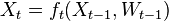
where  models noise on the states, may be nonlinear and time-dependent. The same in general can be said of a function
  relating the evidence to the hidden state.
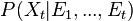
We define the filtering problem as the estimation of the current state value  given the previous state
  and all of the previous pieces of evidence
  . In a regular
bayesian context the estimation of the state is actually a probability distribution:
. In a regular
bayesian context the estimation of the state is actually a probability distribution:
computed in two steps:
These two steps all boil down to integrals, which we don’t expect to be amenable analytically. So what do we do? If we can’t snipe the target then let’s just shoot around at random - that’s the
spirit of the so-called Monte Carlo methods! An option is the bootstrap particle filtering. The particle in it refers to the fact that we
create and maintain a population of random (MC style) particles along the simulation, and bootstrap because it makes use of sampling
with replacement. The point here is that the particles, at every step, represent the state posterior distribution, in the form of a sample rather than a closed form.
It turns out that the algorithm is pretty simple:
-
Extract  samples from the initial prior
  , these are our particles
 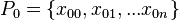 ; these particles are realizations of the variable
-
For each particle in  sample
  , so basically choose how to evolve each sample according to the
  above
above
-
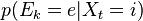
How likely is each evolution? Lookup every score with the evidence function , which is sampling the distribution  ; these values may be one-normalized and represent a weighthing on
the particles population
; these values may be one-normalized and represent a weighthing on
the particles population
-
Bootstrap step, resample with replacement according to the weights; this prepares the population of particles for the next iteration
In the case of discrete distributions, all of the information may be conveniently encoded in matrices and vectors:
Code lines
The code is pretty simple, let’s have a look around with Mathematica. What we want is a program to create and evolve a family of particles, representing the
target distribution, as described above. Let’s stick to an all-discrete world. The signature may simply be:
ParticleFiltering[X_, M_, E_, n_, e_]
where:
-
X is the initial distribution; we are going to generate the first batch of particles from it; if no assumptions may be made then a uniform is always a good prior, but in the particular case of
nice (non-reducible, aperiodic and equipped with an invariant distribution) Markov chains the relevance initial distribution fades away as time goes on
-
M is our transition matrix, in particular M[[i,j]] is the probability of evolving from state i to state j
-
E is the evidence matrix, E[[k,l]] gives us the probability of the hidden state k given that we have seen l as evidence
-
n the number of particles; it should be greater than 30 please!
-
e the vector of recorded evidence scores - this is the information driving our guess for the variable X_t step after step
To simplify things, lets take the support set for the hidden state to be that of natural numbers, so that we can index the matrices easily.
Here is the first generation of particles:
particles = RandomChoice[X -> values, n]
where values is just {0,1,...m}, so we are just randomly choosing from this set enough particles, using the scores of X as weights, we are sampling X
The iteration looks like:
For[i = 1, i <= Length[e], i++,
 For[j = 1, j <= n, j++,
  particles[[j]] = RandomChoice[M[[particles[[j]], All]] -> values];
  weights[[j]] = E[[e[[i]], particles[[j]]]]
 ]
]
so let’s take the row of the M matrix corresponding to the particle value - easy, as the outcome already defines the index - and sample the corresponding line distribution. Rephrased:
- extract a particle
- check what realization is it and seek to the corresponding row on
M
- evolve the particle, thus select a new value at the next instant t+1 based on the row itself, which represents the possible translations
So now say we have evolved from state i to state j, how likely is this to happen given that we know the current evidence sample e_t? We define a number of weights for our newbreed of particles,
right from the evidences:
weights[[j]] = E[[e[[i]], particles[[j]]]]
Now we have a new population of particles, and weights telling us how legitimate they are. Let’s resample it:
particles = RandomChoice[weights -> particles, Length[particles]]
Now repeat!
In general a sampling step is always due in genetic-like algorithms as we know. In the particular procedure here the set of weights might degenerate - a lot of particles might get small weights
rather soon, and we want to get rid of them. On the other side you also run the risk of sample impoverishment - the set is dominated by a few large-weighted particles and we might get steady too soon, missing out on a more fitting particle set.
For a very well written document on this, discussing variations of the basic algorithm too - check out this.
Find the code and some little graphical insights here.
View or add comments
 , we define our hidden state at time
  as a random variable; the process unfolds as an infinite sequence
  of such variables
 . This is the so called memorylessness, we just look at the immediately preceding state to pontificate on the one to come; more precisely the order of the process is how many previous states you take into account
 , in a possibly continuous space, we pass from state
  to state
  with probability
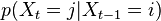
 for every state-evidence pair
  relates state and evidence
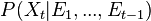 , the prior over
  in the…
 where the value is the probability of transitioning from state
  where the value is the probability of the the observable state
  given the hidden state