Hide that Markov
Carrying particles around
Particle filtering for HMMs
It is a rather common real-life situation one where some piece of information cannot be directly accessed but rather it is inferred by looking at some other information we have, more accessible or readily available. And more often than not, this inference has to be repeated step after step to drive some computation. Very popular examples here are speech recognition and robot movement control:
-
I don’t know exactly what word you are spelling out, but by looking at the waveform it sounds like…
-
our friend the robot does not know where he/she is, though the sensors tell it is quite close to a wall
And very common applications always have very cool, and established, models. The model of reference here is that of hidden Markov models and you can find of course pages galore on the topic. In a nutshell:
-
 , we define our hidden state at time
  as a random variable; the process unfolds as an infinite sequence
  of such variables
 -
Markov rule:
 . This is the so called memorylessness, we just look at the immediately preceding state to pontificate on the one to come; more precisely the order of the process is how many previous states you take into account
 -
Evolution: at every step
for every pair of states  , in a possibly continuous space, we pass from state
  to state
  with probability
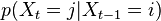
-
At every step we read a value from the indicator variable, whose response is supposed to be meaningfully linked to the hidden state, so something like
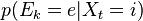 for every state-evidence pair
  relates state and evidence
In the worst case scenarios (read as: always in real-life problems) the evolution probabilities may not be easily estimated:
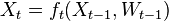
where  models noise on the states, may be nonlinear and time-dependent. The same in general can be said of a function
  relating the evidence to the hidden state.
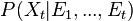
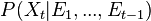
We define the filtering problem as the estimation of the current state value  given the previous state
  and all of the previous pieces of evidence
  . In a regular
bayesian context the estimation of the state is actually a probability distribution:
. In a regular
bayesian context the estimation of the state is actually a probability distribution:
computed in two steps:
-
prediction, calculate
 , the prior over before receiving the evidence score
  in the…
 -
update, the posterior on
is obtained by direct application of the Bayes rule
These two steps all boil down to integrals, which we don’t expect to be amenable analytically. So what do we do? If we can’t snipe the target then let’s just shoot around at random - that’s the spirit of the so-called Monte Carlo methods! An option is the bootstrap particle filtering. The particle in it refers to the fact that we create and maintain a population of random (MC style) particles along the simulation, and bootstrap because it makes use of sampling with replacement. The point here is that the particles, at every step, represent the state posterior distribution, in the form of a sample rather than a closed form.
It turns out that the algorithm is pretty simple:
-
Extract
 samples from the initial prior
  , these are our particles
  ; these particles are realizations of the variable
 -
For each particle in
 sample
  , so basically choose how to evolve each sample according to the
  above
above -
How likely is each evolution? Lookup every score with the evidence function
, which is sampling the distribution  ; these values may be one-normalized and represent a weighthing on
the particles population
; these values may be one-normalized and represent a weighthing on
the particles population -
Bootstrap step, resample with replacement according to the weights; this prepares the population of particles for the next iteration
In the case of discrete distributions, all of the information may be conveniently encoded in matrices and vectors:
-
a matrix
 where the value is the probability of transitioning from state into state
 -
a matrix
 where the value is the probability of the the observable state
  given the hidden state
Code lines
The code is pretty simple, let’s have a look around with Mathematica. What we want is a program to create and evolve a family of particles, representing the target distribution, as described above. Let’s stick to an all-discrete world. The signature may simply be:
ParticleFiltering[X_, M_, E_, n_, e_]
where:
-
Xis the initial distribution; we are going to generate the first batch of particles from it; if no assumptions may be made then a uniform is always a good prior, but in the particular case of nice (non-reducible, aperiodic and equipped with an invariant distribution) Markov chains the relevance initial distribution fades away as time goes on -
Mis our transition matrix, in particularM[[i,j]]is the probability of evolving from stateito statej -
Eis the evidence matrix,E[[k,l]]gives us the probability of the hidden statekgiven that we have seenlas evidence -
nthe number of particles; it should be greater than 30 please! -
ethe vector of recorded evidence scores - this is the information driving our guess for the variableX_tstep after step
To simplify things, lets take the support set for the hidden state to be that of natural numbers, so that we can index the matrices easily.
Here is the first generation of particles:
particles = RandomChoice[X -> values, n]
where values is just {0,1,...m}, so we are just randomly choosing from this set enough particles, using the scores of X as weights, we are sampling X
The iteration looks like:
For[i = 1, i <= Length[e], i++,
 For[j = 1, j <= n, j++,
  particles[[j]] = RandomChoice[M[[particles[[j]], All]] -> values];
  weights[[j]] = E[[e[[i]], particles[[j]]]]
 ]
]
so let’s take the row of the M matrix corresponding to the particle value - easy, as the outcome already defines the index - and sample the corresponding line distribution. Rephrased:
- extract a particle
- check what realization is it and seek to the corresponding row on
M - evolve the particle, thus select a new value at the next instant t+1 based on the row itself, which represents the possible translations
So now say we have evolved from state i to state j, how likely is this to happen given that we know the current evidence sample e_t? We define a number of weights for our newbreed of particles,
right from the evidences:
weights[[j]] = E[[e[[i]], particles[[j]]]]
Now we have a new population of particles, and weights telling us how legitimate they are. Let’s resample it:
particles = RandomChoice[weights -> particles, Length[particles]]
Now repeat!
In general a sampling step is always due in genetic-like algorithms as we know. In the particular procedure here the set of weights might degenerate - a lot of particles might get small weights rather soon, and we want to get rid of them. On the other side you also run the risk of sample impoverishment - the set is dominated by a few large-weighted particles and we might get steady too soon, missing out on a more fitting particle set.
For a very well written document on this, discussing variations of the basic algorithm too - check out this.
Find the code and some little graphical insights here.